
Network Analysis of EEG data
Network Analysis of EEG data

Introduction
This tutorial will use calculate common graph theory metrics on EEG data. We will use several high-quality toolboxes to create a straightforward, transparent workflow to use on your own data.
Our lab primarily processes and stores files using the SET (EEGLAB) format. Our custom toolbox, vHTP, primarily uses SET structures as inputs and outputs. Our workflow will start with a SET EEG file and ultimately end up with a CSV of graph results we can import into R (or other stats program) to perform statistics.
Overview
The readily available graph theory toolboxes primarily use GUI-style interfaces to process data. Though this has some advantages, it is difficult to quickly reproduce and work with batches.
Our general plan:
Load source-localized EEG data
Compute various connectivity matrices (phase (wpli), coherence (coh), and synchronization likelihood (SL).
generate weighted undirected (WU) and binary undirected (BU) brain graphs of the connectivity matrices.
Compute global and nodal graph measures
We will do this on a subject-by-subject basis and then combine our findings into a large table.
Resources and Prerequisites
vHTP toolbox: https://github.com/cincibrainlab/vhtp
eeglab: https://github.com/sccn/eeglab
FastFc: https://github.com/juangpc/FastFc
Braph 1.0: https://github.com/softmatterlab/BRAPH
Hermes Toolbox: https://github.com/guiomar/HERMES
We are using MATLAB 2022 with the signal processing toolbox.
1. Loading source localized EEG data
Due to inherent limitations of scalp level EEG data, most connectivity analysis is recommended to be performed at the source level. In our lab, we usually collected 128-channel EEG data through EGI/Magstim equipment. We have streamlined the construction of minimal norm estimate (MNE) models (with default electrode and averaged adult MRI) using Brainstorm. A single function, eeg_htpCalcSource, can create an EEGLAB-style SET file containing 68 DK-atlas regions (via Brainstorm) as channels from a preprocessed 128-channel EEG SET file. The function can be modified to use individual head models, different electrode montages, or head models.

For this tutorial, I will be working off of pre-existing source localized SET files available here.
% load source-localized EEG dataset
sEEG = pop_loadset('filename', 'D0079_rest_postcomp.set', 'filepath', data_folder);
sEEG.data = double(sEEG.data);
This file consists of 68 “channels” or atlas nodes with about 80 seconds of continuous data for each channel. It is extremely important to make sure your data values are in double, otherwise you will notice lots of zeros and NaNs in your calculations as small values are rounded to 0 in single precision mode.
2. Calculate various connectivity matrices
It is no secret that graph measures can be intimidating. Before thinking about what a graph measure means, it is important to identify what the graph measure is being calculated on. I often remind learners that there is no general “graph” measure of an EEG, it must be based on a pre-existing connectivity feature. When presenting graph-based measures, it is also important to ensure the audience understands what the underlying feature was. I have heard entire professional talks where graph theory results were presented without any clear hint to what EEG feature was being measured!
For this tutorial I have selected three connectivity features to estimate for each EEG file:
The weighted phase lag index (wpli) is an undirected phase-based measure of connectivity.
Spectral coherence (coh) is an undirected normalized covariance of two time series in the frequency domain
Synchronization likelihood (SL) the concept of generalized synchronization and detects nonlinear and linear dependencies between two signals.
There are many implementations of these methods, but my preference is to use efficient methods to cut down on computational time (which can be significant for large datasets).
The result of any of these functions will be an atlas node (channel) by atlas node (channel) square matrix with rows serving as “from” and the columns as “to”. Since these are undirected measures, the matrix will be symmetric. The diagonal will be “0” since nodes do not have connections to themselves.
Proof of concept using Phase Lag Index
Let’s start with calculating wPLI for a single subject and calculating some graph based measures.
After loading the data, we will have to filter the data to the frequency band of interest. I would like to look at three bands: theta, alpha2, and gamma1. Let’s define these bands in a simple cell array to use later:
freqbands = {'theta', [5 7]; 'alpha2', [10 12]; 'gamma1', [30 57]};
Filter by Frequency Band
To filter the data, I have a custom function which implements either the FastFc (matlab c-compiled). If you do not have this toolbox installed, it will default to the MATLAB filtfilt function which requires the signal processing toolbox. I have found these filters be similar in quality to implementation in EEGLAB (firfilt) but an order of magnitude faster. An example line of code to filter the alpha band:
[fEEG] = eeg_htpEegFilterFastFc( sEEG, 'bandpass', [10 12] );Let’s create a simple loop to accomplish this and store each into a structure designated by bandname. I have also added an epoch function to divide the filtered continuous function into 2-second epochs:
% filter by frequency band
for fi = 1 : length(freqbands)
    fEEG.(freqbands{fi,1}) =  ...
        eeg_htpEegCreateEpochsEeglab( ...
        eeg_htpEegFilterFastFc( ...
            sEEG, 'bandpass', freqbands{fi,2} ));
end

Channel Labels
Let’s also grab the channel labels which we will need to use to interpret our matrices and graph measures:
chanlabels = {fEEG.chanlocs.labels};wPli Connectivity Matrix
Let’s add our wpli function into the loop and generate our connectivity matrices:
% filter by frequency band
% create regular epochs for resting state data
for fi = 1 : length(freqbands)
    fEEG.(freqbands{fi,1}) =  eeg_htpEegCreateEpochsEeglab( ...
        eeg_htpEegFilterFastFc( sEEG, 'bandpass',      freqbands{fi,2} ));
    wpli.(freqbands{fi,1}) = fastfc_wpli( ...
        eeg_htpCalcReturnColumnMatrix( ...
         fEEG.(freqbands{fi,1}) ...
        ));
end
The code of interest uses the fastfc_wpli function to store the results of the connectivity matrix (68 x 68) for each frequency band filtered EEG structure into a new structure called wpli.

Let’s also add some visualization code to the loop:
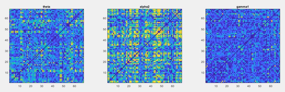
% filter by frequency band
% create regular epochs for resting state data
figure;
axis square;
for fi = 1 : length(freqbands)
    fEEG.(freqbands{fi,1}) =  eeg_htpEegCreateEpochsEeglab( ...
        eeg_htpEegFilterFastFc( sEEG, 'bandpass', freqbands{fi,2} ));
    wpli.(freqbands{fi,1}) = fastfc_wpli( ...
        eeg_htpCalcReturnColumnMatrix( ...
         fEEG.(freqbands{fi,1}) ...
        ));
    subplot(1,3,fi);
    imagesc( wpli.(freqbands{fi,1}) );
    axis square;
    axis xy;
    title(freqbands{fi,1})
end
Network Measures using the Braph Toolbox
The Braph toolbox (https://github.com/softmatterlab/BRAPH) is a particularly straightforward set of scripts to generate network measures. The included manual is also a straightforward introduction to graph-based measures. This manual with chapter 31 (Graph Theory) of Cohen’s Analyzing Neural Time Series Data I think is sufficient to interpret and understand most graph theory manuscripts.
Let’s discuss a little background before performing graph theory measures.
brain connectivity matrix (BCM): generally the BCM involves a measure of connection strength between brain regions. The details differ based on the neuroimaging modality.
structural versus functional data: Structural BCMs provide a single value for a subject that is correlated across a group. This may include MRI/PET measures such as cortical thickness, glucose metabolism, or spectroscopy. The connection strength is the correlation of values between two regions across the group. Ultimately, this will provide a single BCM for each group. On the other hand, a functional BCM measures connection strength between two regions as a function of time. A functional BCM can be made for each subject.
In this tutorial we will be generating graph measures based on:
Data type: functional data from EEG
BCM: phase-based measures, weighted phase lag index (wPLI)
Graphs
A graph consists of nodes connected by edges. In our data, nodes represent source-localized EEG regions (parcellated with an atlas). The edges represent the wPLI connection strength between the nodes. The BCM is a convenient way to represent a graph - the rows (x) and columns (y) represent the nodes and each value (x,y) within the matrix represents the edge (wPLI in the figures above). In some cases, the direction of the connection matters - the strength of node A to node B is different than the strength of node B to node A. In this case, by convention, the columns represent the outgoing connections. A train station analogy can be helpful - each row node represents the origin city and the columns of the matrix are the destination cities.
Types of Graphs
There are four types of graphs you can create from this basic information.
Undirected (U) versus directed (D): First a graph can be undirected or directed. This refers if the reverse connection strength is different than the forward direction. This also includes the possibility that a node may be connected to another node, without a reverse connection. An undirected graph can be made from a directed graph via symmetrization (i.e. averaging connection strengths of each direction).
Weighted (W) or Binary (B): The other high-level distinction is that a BCM may either use the actual weights (or a continuous value) or either indicate the presence (1) or absence (0) of a connection. The latter is known as a binary graph. A binary graph can be constructed from a weighted graph.
Thus, we have four possible types of basic graphs: WU, WD, BU, or BD. Which one applies to your data is determined by the type and nature of the underlying BCM.
Considering our dataset
Our underlying BCM is based on EEG regions and wPLI connection strengths. This particular measure is weighted undirected (WU) - the strength is a real number and the same from each node to another and the reverse.
A weighted graph can be converted to a binary graph by defining a certain threshold which can be used to define if an edge is true (1) or false (0). Obviously, the thresholding value is a matter of great care - it can be defined ahead of time or empirically, but will substantially impact your results and how you can compare graphs across a group or time. Alternatively, you may want to have a variable threshold that generates a BCM where there is a similar density of “true” edges with other BCMs.
In this tutorial, we will start with analyzing our data as a WU and then examine a few thresholding strategies to generate BUs.
Types of Graph Measures
To start, there are two categories of graph measures - global (representing a single value per a graph) and nodal (representing a single value per a node). We will implement the measures provided by the Braph toolkit manual presented on page 23 of the manual.
How Braph functions are used. Braph functions implement object-oriented programming in MATLAB, so the syntax may be a little unusual from what you are used to. For each function, the Braph authors included a “test” function that provides a self-contained example.
Let’s start with the basic syntax:
% Implementation of Braph Functions
% add braph toolkit to the path
bandlabels =  fieldnames(coh);
for ib = 1 : numel(fieldnames(coh))

    current_bcm = coh.(bandlabels{ib});

end
Though there is a little extra complexity upfront to set up a loop, given that we have created three BCM based on frequency bands, we can examine the strength and compare between bands. The current_bcm is the pure numerical matrix generated by the connectivity function. In this case, the diagonals are NaNs. We will replace this with 0s (no self-edges with nodes).
Let’s now incorporate Braph into our loop. We will first create a Braph graph object (WUgraph). Next we run node and global strength graph measure for each BCM by frequency band.
bandlabels =  fieldnames(coh);
for ib = 1 : numel(fieldnames(coh))

    current_bcm = single( coh.(bandlabels{ib}) );
    WUgraph = GraphWU(current_bcm);

    %% Calculate the strenght from Graph
    node_strength.(bandlabels{ib}) = WUgraph.strength();
    glob_strength.(bandlabels{ib}) =   WUgraph.measure(Graph.STRENGTHAV);

end
To visualize these results, we can plot strength by node and use colors to represent different bands:

The x-axis contains the 68 regions (in alphabetical order). The atlas node are the more fine-grained level at which to look at data. We could use either functional or regional labels to group results and reduce the number of points.
Plot code:
figure('color','w');
for ib = 1 : numel(fieldnames(coh))
    if ib == 1
        plot(nodelabels, node_strength.(bandlabels{ib}))
        hold on;
    else
        plot(nodelabels, node_strength.(bandlabels{ib}));
    end
end
legend(bandlabels);
xlabel("Atlas Region")
ylabel("Nodal Strength")
Let’s take a shot at an interpretation:
Higher wpli values indicate a greater synchronization of phases between the time series between regions (with some accounting for volume conduction). Between the three frequency bands, there are regions with similar strengths - but several regions in which high-frequency power has lower strength than low-frequency bands (theta / alpha2).
Let’s also look at global strength:

Plot code:
figure('color','w');
subplot(2,1,1)
for ib = 1 : numel(fieldnames(coh))
        subplot(2,1,1)
        plot(nodelabels, node_strength.(bandlabels{ib}))
        legend(bandlabels);
        xlabel("Atlas Region")
        ylabel("Nodal wPLI Strength")
        hold on;
        subplot(2,1,2)
        bar(categorical(bandlabels(ib)), mean(node_strength.(bandlabels{ib})))
        xlabel("Frequency Band")
        ylabel("Global wPLI Strength (Mean + SD")
        hold on;
        errorbar(categorical(bandlabels(ib)), mean(node_strength.(bandlabels{ib})), std(node_strength.(bandlabels{ib})), 'k')
end
Conclusion and Next Steps
In this post we looked at using the Braph toolbox in an EEG SET file workflow to calculate graph measures. In the next post, I will be introducing a ready made function that calculates a set of complete measures from an EEG SET file.